Hierarchical Clustering with MPDist

In this tutorial you will see how to use the novel MPDist metric to cluster time series data. The time series data used in this example is accelerometer data consisting of individuals performing the following actions:

1. Working at Computer

2. Standing Up, Walking and Going updown stairs

3. Standing

4. Walking

5. Going UpDown Stairs

6. Walking and Talking with Someone

7. Talking while Standing

You can read more about the data set here:

http://archive.ics.uci.edu/ml/datasets/Activity+Recognition+from+Single+Chest-Mounted+Accelerometer

In essence, MPDist considers “…two time series to be similar if they share many similar subsequences, regardless of the order of matching subsequences.” [1] I encourage those interested in the details of the metric to read the paper.

Note that all code written in this tutorial has only been tested with Python 3!

import pandas as pd
import numpy as np
import matrixprofile as mp
from scipy.cluster.hierarchy import dendrogram

from matplotlib import pyplot as plt

%matplotlib inline

Download and Extract Data

In this section we simply obtain the dataset and extract it.

import urllib.request
import zipfile
import tempfile
import os

temp_dir = tempfile.mkdtemp()
url = 'http://archive.ics.uci.edu/ml/machine-learning-databases/00287/Activity%20Recognition%20from%20Single%20Chest-Mounted%20Accelerometer.zip'
tmp_file = os.path.join(temp_dir, 'activity_recognition.zip')
extracted_dir = os.path.join(temp_dir, 'extracted')

os.makedirs(extracted_dir, exist_ok=True)

with urllib.request.urlopen(url) as response, open(tmp_file, 'wb') as out_file:
    data = response.read() # a `bytes` object
    out_file.write(data)

with zipfile.ZipFile(tmp_file, 'r') as zip_ref:
    zip_ref.extractall(extracted_dir)

data_dir = os.path.join(extracted_dir, 'Activity Recognition from Single Chest-Mounted Accelerometer')

Load Raw Data

In this section we load the raw data and process it. For readability purposes, the target labels are transformed into human readable descriptions.

label_description = '''
1: Working at Computer
2: Standing Up, Walking and Going updown stairs
3: Standing
4: Walking
5: Going UpDown Stairs
6: Walking and Talking with Someone
7: Talking while Standing
'''

labels = []

for line in label_description.split('\n'):
    line = line.strip()
    if line == '':
        continue

    tmp = line.split(':')
    num = tmp[0].strip()
    description = tmp[1].strip()

    labels.append({
        'label': str(num),
        'description': description
    })

labels_df = pd.DataFrame(labels)

labels_df

	label	description
0	1	Working at Computer
1	2	Standing Up, Walking and Going updown stairs
2	3	Standing
3	4	Walking
4	5	Going UpDown Stairs
5	6	Walking and Talking with Someone
6	7	Talking while Standing

This code snippet reads all of the csv files with pandas and combines them into a single data frame.

from glob import glob

dfs = []

for csv in glob(os.path.join(data_dir, '*.csv')):
    df = pd.read_csv(csv, header=None, names=['sequence', 'x', 'y', 'z', 'label'])
    df['label'] = df['label'].astype('str')
    df['participant_id'] = csv.split('/')[-1].replace('.csv', '')
    df = pd.merge(df, labels_df, on='label')
    dfs.append(df)

df = pd.concat(dfs)

df

	sequence	x	y	z	label	participant_id	description
0	0.0	1983	2438	1825	1	11	Working at Computer
1	1.0	1948	2442	1797	1	11	Working at Computer
2	2.0	1927	2388	1784	1	11	Working at Computer
3	3.0	1960	2319	1831	1	11	Working at Computer
4	4.0	1967	2274	1871	1	11	Working at Computer
...	...	...	...	...	...	...	...
122195	122200.0	2063	2360	2000	7	4	Talking while Standing
122196	122200.0	2056	2368	2001	7	4	Talking while Standing
122197	122200.0	2059	2366	2001	7	4	Talking while Standing
122198	122200.0	2063	2382	2004	7	4	Talking while Standing
122199	122200.0	2071	2381	2004	7	4	Talking while Standing

1923177 rows × 7 columns

The data consists of multiple coordinates from the accelerometer readings. Here we will just use the x data point.

cols = ['sequence', 'x', 'label', 'participant_id', 'description']

df = df[cols].copy()

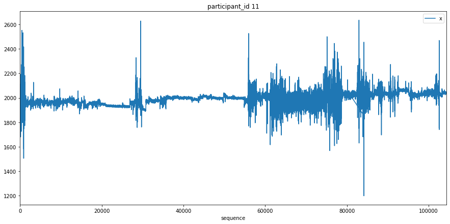
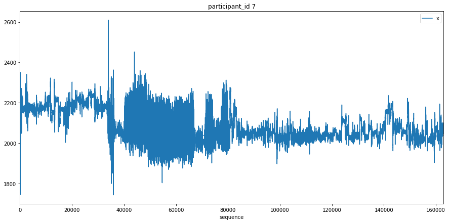
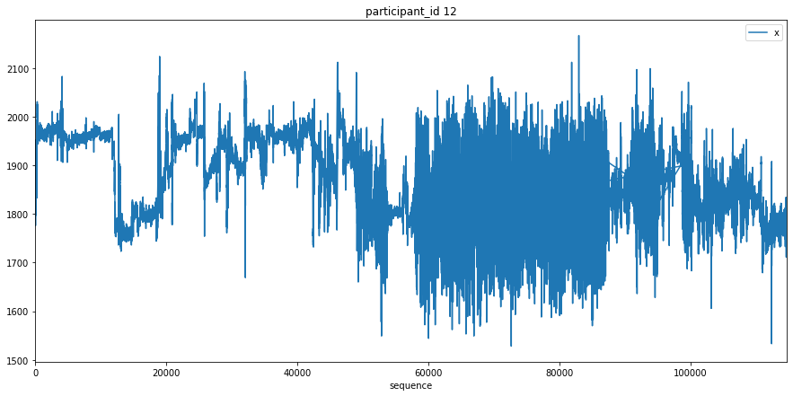
Visualize Participant Data

Here we just plot the entire x signal for a few participants to get an understanding of what the data looks like.

c = 0
for participant_id in df['participant_id'].unique():
    c += 1
    df[df['participant_id'] == participant_id].plot(x='sequence', y='x', title=f'participant_id {participant_id}', figsize=(15, 7))
    plt.show()

    if c >= 3:
        break

Transform Data

This section transforms the data so that we have subsequences of data corresponding to a given activity. The series_data array contains the subsequences of an activity, the series labels are used to keep track of the activity, and the participant labels are used to keep track of the participant.

df = df.sort_values(['participant_id', 'sequence'])

series_data = []
series_labels = []
participant_labels = []

for idx, items in labels_df.iterrows():
    descr = items['description']
    label = items['label']

    for participant_id in df['participant_id'].unique():
        mask = (df['participant_id'] == participant_id) & (df['label'] == label)
        values = df[mask]['x'].values

        series_data.append(values)
        series_labels.append(descr)
        participant_labels.append(participant_id)

len(series_data[0]), series_labels[0], participant_labels[0]

(33677, 'Working at Computer', '1')

Random Sampling

Here we take 25 random samples from the data set to see if our clustering seems logical. This saves time in the exploration phase allowing you to test more parameters.

np.random.seed(9999)
random_indices = np.random.choice(np.arange(105), size=25, replace=False)

random_samples = []
random_labels = []

for random_index in random_indices:
    random_samples.append(series_data[random_index])
    random_labels.append(series_labels[random_index])

Good Enough Window Size

Here we look identify what a “good” window size may be based on the minimum length of the time series. The window size must be smaller than the smallest time series length for the MPDist calculation to work.

lengths = []

for ts in random_samples:
    lengths.append(len(ts))

np.min(lengths)

928

Clustering and Visualizing Results

Now that all of the data processing is complete, we can finally cluster the sampled data and look at the results.

clusters = mp.discover.hierarchical_clusters(random_samples, 128, 2, n_jobs=8)

dendrogram(clusters['linkage_matrix'], labels=random_labels, leaf_rotation=90)
plt.show()

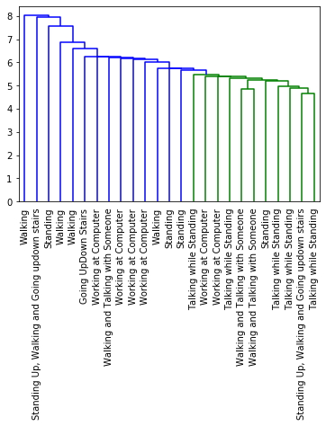
The results seem logical, however the dataset used uncalibrated accelerometers and I only chose to use the x value. I do not know if the x value is representative enough to identify all activities. With this in mind, I encourage you to take this example and test it on the z or y value and even toy with the clustering parameters.

Citations

1. Matrix Profile XII: MPdist: A Novel Time Series Distance Measure to Allow Data Mining in More Challenging Scenarios. Shaghayegh Gharghabi, Shima Imani, Anthony Bagnall, Amirali Darvishzadeh, Eamonn Keogh. ICDM 2018. expanded version PDF